
Creating a Hex Scatterplot in Tableau

I recently came across a brilliant data visualization by The Guardian that seeks to help you understand how populist you are. After answering a number of political questions, it creates a hexagonal scatterplot showing where you fall on a spectrum of populist to not populist and left to right (liberal to conservative). For example.
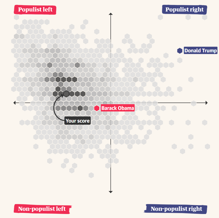
I loved this chart, primarily because, unlike a normal scatterplot, it bins the data so you can see the hotspots of people who took the quiz. This provides some insight immediately, such as the fact that a much higher proportion of the people tend to be more left-leaning and somewhere in the middle of the populism spectrum.
Creating it in Tableau
So, considering how well the chart worked in this scenario, I wanted to see if I could build it in Tableau.
Note: If you’re not interested in all the technical details of how to build this, then feel free to skip to the end of this post where I share a plug-and-play template.
Conceptually, we’d have to do the following:
- Bin our two measures.
- Move every other row in ½ of our bin size in order to create the tessellation.
- Plot each point using a hexagon.
Sounds simple, right?
I decided to use a data set provided by Jacob Olsufka from PitchFX which shows the location of pitches thrown in Major League Baseball last year. I chose this data set for a couple of reasons. First, it should show some clear hotspots. Second, the X and Y axes represent spatial distances, so one unit on the X axis is the same as one unit on the Y axis. Other than that, the data itself isn’t particularly important and I won’t be focusing too much on analyzing it.
Note: For simplicity, I’ve named the my X axis measure Measure X and my Y axis measure Measure Y.
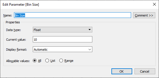
I wanted to make the bin size a user-configurable option, so I started by creating a Bin Size parameter.
Because my bin size is configurable, I can’t use Tableau bins and needed to bin the measures via a calculated field. So I used a BYO Bin technique developed by Joe Mako, which I learned by way of Jonathan Drummey. (Quick note: This technique is quite powerful as it opens up a number of capabilities that can’t be done with normal bins, so be sure to check it out.) The formula Joe provides is:
INT([Value]/[Bin Size])*[Bin Size]-IIF([Value]<0,[Bin Size],0)
Applied to my data, it looks like this:
Measure X Bin
INT([Measure X]/[Bin Size])*[Bin Size]-IIF([Measure X]<0,[Bin Size],0)
Measure Y Bin
INT([Measure Y]/[Bin Size])*[Bin Size]-IIF([Measure Y]<0,[Bin Size],0)
But, as noted previously, we need to adjust the X coordinate so that every other row is pushed in by ½ of a bin, which will allow use to tessellate our hexagons. So, we’re going to throw out the above Measure X Bin calculation. Instead, we’ll first make some adjustments to the Measure X to handle or “indentation” based on whether we’re on an odd or even row (based on Measure Y Bin):
Measure X Adjusted
// To create the tessellation after creating bins, we need to make slight adjustments to the measure.
IF ([Measure Y Bin]/[Bin Size])%2 = 0 THEN
// Even numbered row. Adjust forward.
[Measure X]+([Bin Size]/2)-1
ELSE
// Odd numbered row. Don't adjust.
[Measure X]-1
END
Then we’ll create bins on this field.
Measure X Bin Adjusted
// Calculate the bin of the adjusted measure and indent.
IF ([Measure Y Bin]/[Bin Size])%2 = 0 THEN
// Even numbered row.
INT([Measure X Adjusted]/[Bin Size])*[Bin Size]-IIF([Measure X Adjusted]<0,[Bin Size],0)
ELSE
// Odd numbered row. Push the bin forward by half the bin size.
INT([Measure X Adjusted]/[Bin Size])*[Bin Size]-IIF([Measure X Adjusted]<0,[Bin Size],0) + [Bin Size]/2
END
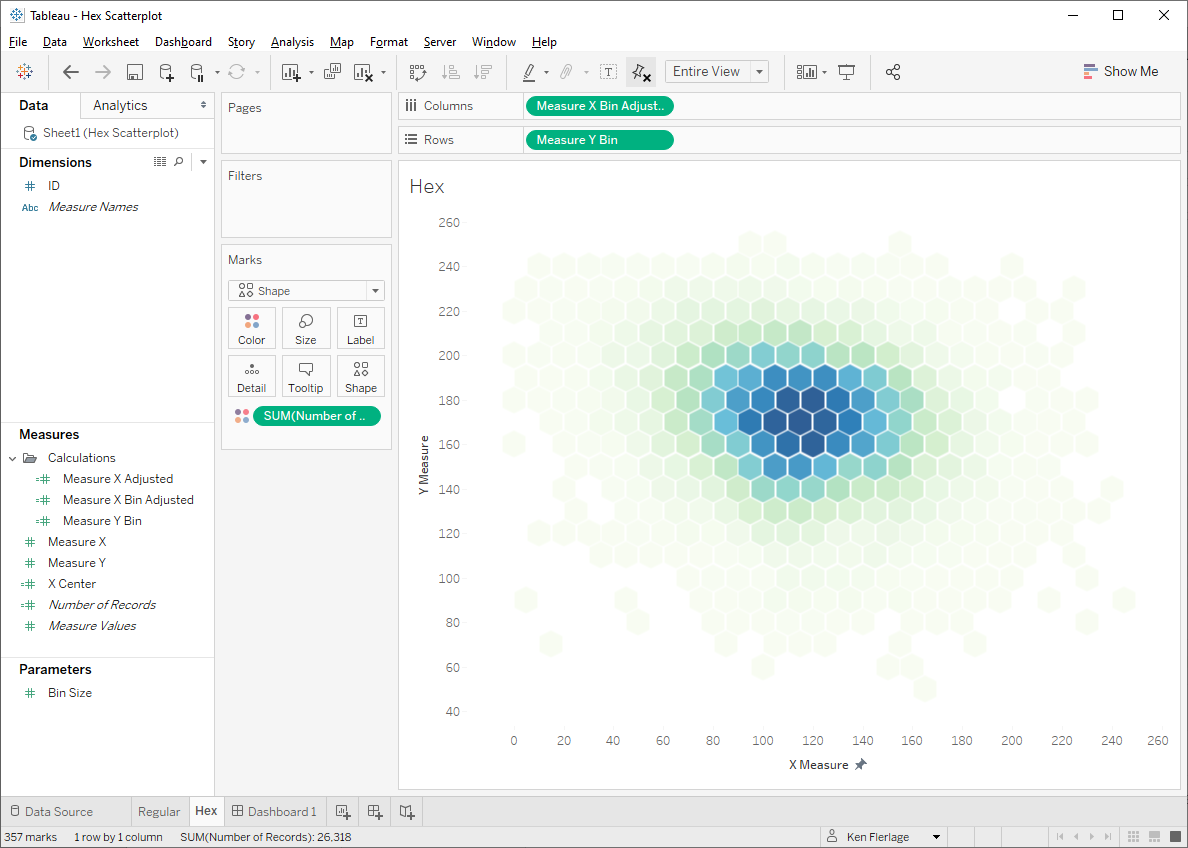
Next I created a scatterplot using these measures and colored by the number of records:

Looks pretty good just like that, doesn’t it!
But I wanted hexagons, so I simply changed the mark type to shape and selected a hexagon.
This was exactly what I wanted! So I added it to a dashboard and…
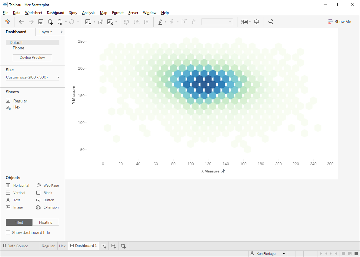
Okay, this is NOT what I wanted. The problem is that shape sizes cannot be fixed so they will stay the same size even if you resize the chart. So, to get this right we’d have to adjust the height and width of the chart on the dashboard, then switch to the sheet and fiddle with the shape size until we got it just right.
This is not a new problem with hexagon shapes, of course. Due to this exact same problem with hex maps, a couple of years ago, we saw a spate of innovation with them that led to the creation of polygon hex maps by Rody Zakovichand a hex map spatial file by Joshua Milligan.
Polygonizing It!
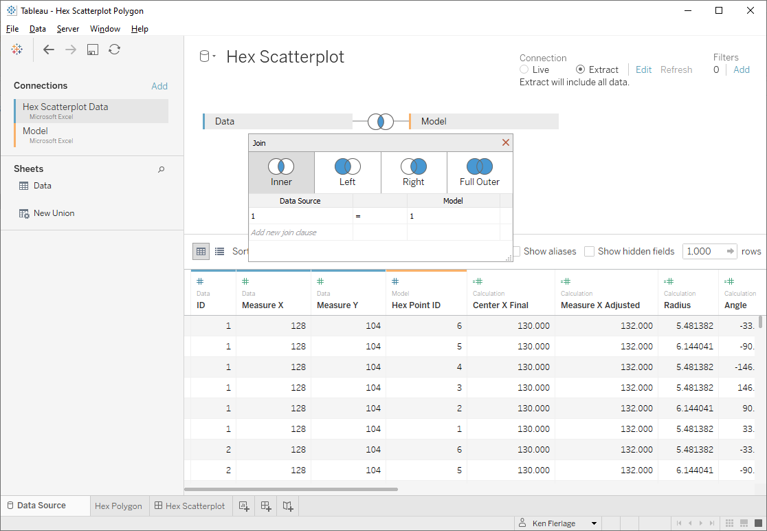
So, let’s see if we can change this to use polygons instead of hexagon shapes. To do this, we’ll need six points for each hexagon, so I created a “Model” data set that includes a single column with six rows:

Now we’ll cross-join the model to our data (for more on cross joins, see SQL for Tableau Part 2: Combining Data).
Now we will draw the hexagons. We want these hexagons to be regular (i.e. each side is the same length and all the inner angles are the same). To do this, we can just draw a circle with 5 points. That’s right, a regular polygon uses the exact same math as drawing a circle, just with a reduced number of points. In fact, when drawing circles in Tableau (or any software, for that matter), we’re never actually drawing a circle, but rather we are drawing a regular polygon with so many points that it looks like a smooth circle.
To draw these regular hexagons using trig, we need two pieces of information—the angle of each point and the radius. Let’s start with the angle. A hexagon has 6 points and we want to space the angle out starting at 0° and moving around radially 360°. So the angle spacing will be 360/6 or 60. So, to get the angle, we can use a calculated field like this:
Angle
// Space each point by 60°
([Hex Point ID]-1)*60
Point 1 will be at 0°, point 2 at 60°, point 3 at 120°, etc.
As we want our hexagons to fill in each bin, the radius will be half the bin size.
Radius
// We want our radius to be 1/2 of the bin size.
[Bin Size]/2
Then we use COS and SIN calculations to get the X and Y coordinates (For more on using trig to determine X and Y coordinates, see Beyond "Show Me" Part 2: Trigonometry).
But there’s a problem here. The rotation of our hexagons do not allow for proper tessellation. Thus we need to rotate them so that there is a point at the top and bottom. To do this, we just need to adjust our angle by 30°.
Angle
// Space each point by 60°
([Hex Point ID]-1)*60-30

OK, we have the right positioning of our hexagons now, but the size isn’t quite right to get tight tessellation. This is because our radius is not quite accurate. So let’s create a parameter that will allow us to adjust the size to get a better fit. We can then multiply the radius by this value.
Radius
// We want our radius to be 1/2 of the bin size.
// Adjust the size in order to create tighter tessellation.
[Bin Size]/2*[Size Adjustment]
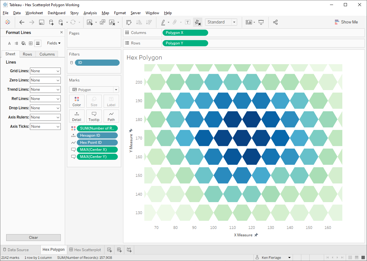
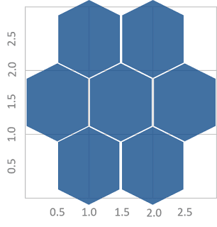
Getting closer, but there’s still a problem. The hexagons overlap horizontally while leaving quite a bit of space vertically. So what’s going on here? The problem is that, while the hexagons themselves are taller than they are wide, the tessellation of each hexagon with the rows above and below has the opposite effect, making them consume less space vertically than horizontally. To explain this better, see the following visual which tightly tessellates regular hexagons on a 3 x 3 grid.
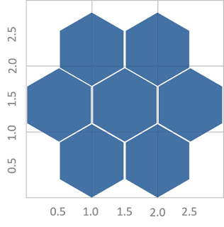
Our goal would be that each hexagon takes up a 1 x 1 space on the grid, but as you can see, the vertical tessellation causes this to not happen and space gets “lost” the higher we go vertically.
One option to fix this would be to adjust our Y axis so that the hexagons do fit nicely, but in my opinion, that would be an act of visual dishonesty as one unit on the Y axis would be visually smaller than one unit on the X axis. So, instead of this approach, I decided to stretch the hexagons slightly so that they fit nicely into 1 x 1 grids.
To do this, we’ll need to adjust the radiuses and angles of each point slightly. I worked out the math and ended up with the following for the angle:
Angle
// We'll draw a hexagon by drawing a circle with 6 points.
// However, to get them to tessellate properly, without adjusting the axes...
// ...we'll make them slightly taller than a regular polygon.
CASE [Hex Point ID]
WHEN 1 THEN 33.5
WHEN 2 THEN 90
WHEN 3 THEN 146.5
WHEN 4 THEN -146.5
WHEN 5 THEN -90
WHEN 6 THEN -33.5
END
And the following for radius.
Radius
// // We'll draw a hexagon by drawing a circle with 6 points.
// However, to get them to tessellate properly, without adjusting the axes...
// ...we'll make them slightly taller than a regular polygon.
IF [Hex Point ID]=2 OR [Hex Point ID]=5 THEN
([Bin Size]*1)/2*[Size Adjustment]
ELSE
([Bin Size]*1)/2*[Stretch Factor]*[Size Adjustment]
END
Note: Stretch Factor is a new parameter I created to allow us to adjust the width of the hexagons.
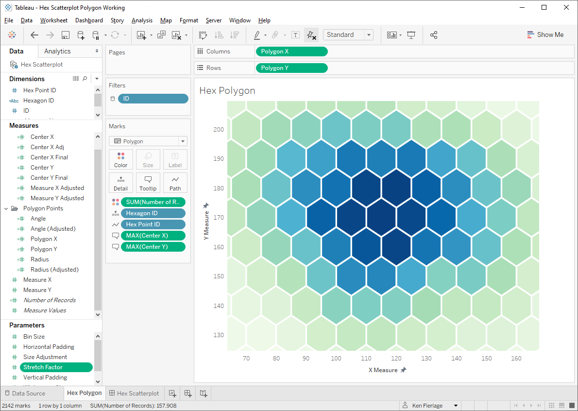
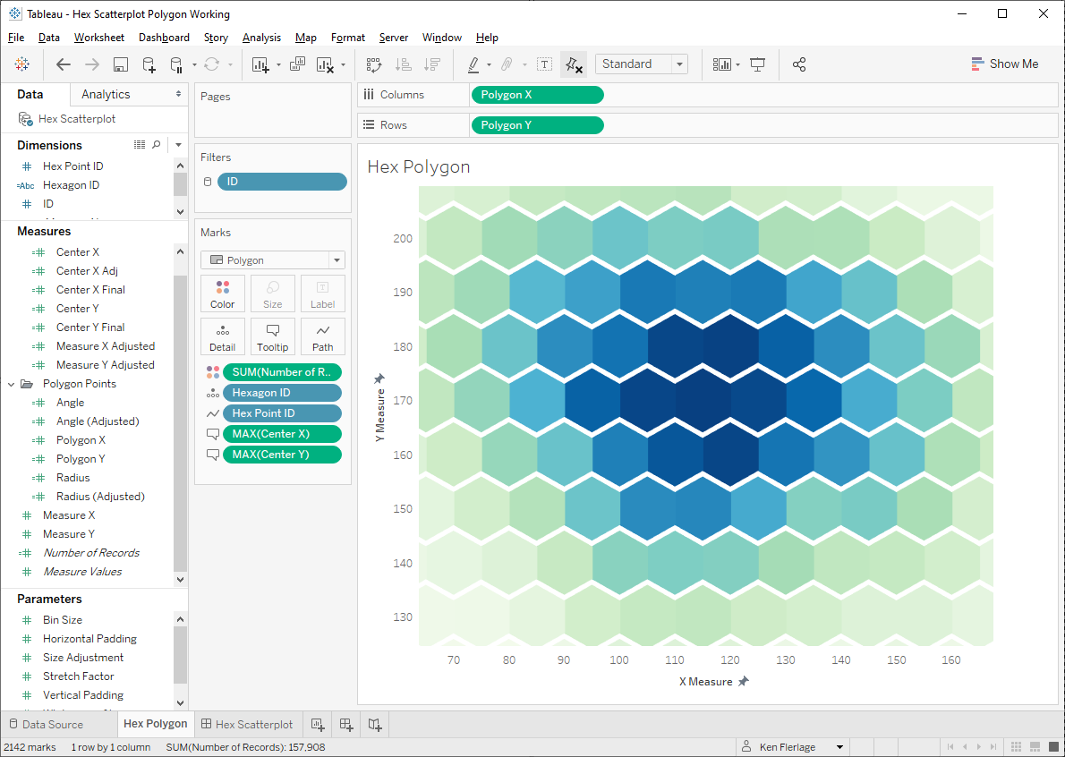
Alright!! That’s what we were looking for! The hexagons now tessellate nicely while not requiring any squishing of the Y axis.
I should note here that my final workbook included one more parameter not mentioned above, Whitespace. This allows you to adjust the spacing in between the polygons. So, if desired, you can increase the
Reusable Template
This was tricky to create and, while there may only be niche use cases, I thought it would be good to templatize it so that people can easily plug in their own data. As with all of my templates, this one includes two components—an Excel spreadsheet and a Tableau workbook.
The Excel spreadsheet has two sheets, Data and Model. Model is used to handle the polygon points. You don’t need to modify this sheet at all; just make sure it’s in your spreadsheet. The Data sheet will be used to populate your actual data. It contains just three columns. You can add more if needed, but these are the three that are required by the Tableau template. The columns are as follows:
ID – Unique numeric identifier for each record.
Measure X– Measure that will be plotted on the X axis of the scatterplot.
Measure Y– Measure that will be plotted on the Y axis of the scatterplot.
Once you have populated the Data sheet, then you need to connect it to Tableau. Start by downloading the template Tableau workbook from my Tableau Public page. Then edit the data source and connect it to your Excel template. The workbook should update automatically to reflect your data.
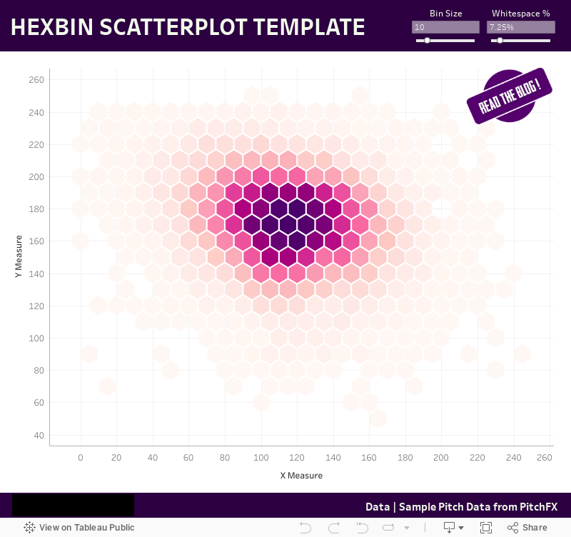
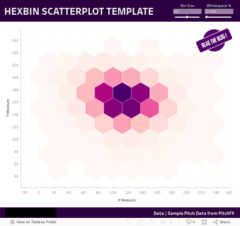
As noted earlier, the template allows you to change the bin size. For example, here’s my sample data using a bin size of 10.
And here it is using a bin size of 25:
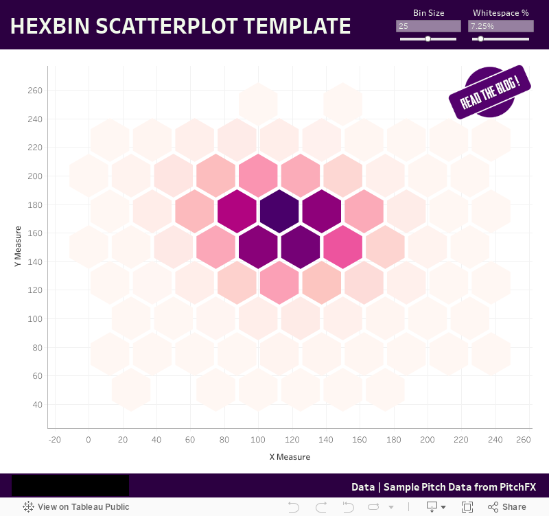
Adjusting the bin size allows you to sort of zoom in or out of the data as desired.
Also, as noted above, you can adjust the whitespace in order to control the spacing between polygons. For example, the following shows 0% whitespace:
And here it is with 15% whitespace.
Once you have everything adjusted to fit your needs, you can make whatever other changes you desire—change the colors, add filters, update tooltips, etc. just as you normally would.
And that’s all there is to it. If you use this template to create your own hex scatterplot, I’d love to see it.
Thanks for reading!!
Ken Flerlage, September 8, 2019


No comments: